


Lesson overview

Learn to clean data in preparation for visualization.
In the previous lesson, Google Sheets: Scraping data from the internet, we learned how to import a table from the Web using importHTML. In this lesson, we'll learn how to clean the data so it’s ready for analysis and visualization.
- Making data editable.
- Editing the data.
- Batch editing with Find and replace.
For more Data Journalism lessons, visit:
newsinitiative.withgoogle.com/training/course/data-journalism
Making data editable.
“Cleaning data” means making it usable to work with: ensuring a table has integrity, is free from inconsistencies and is structured in a way that computers will understand. That means we will remove duplicate rows, delete undesired characters and ensure that columns hold only one type of data, for example numbers or text, but not both. First, we need to make the data editable.
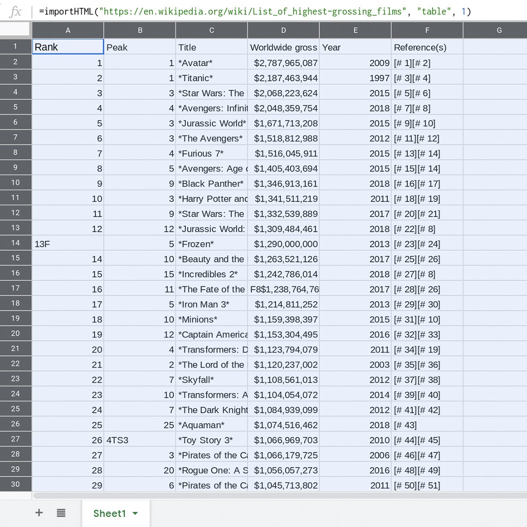
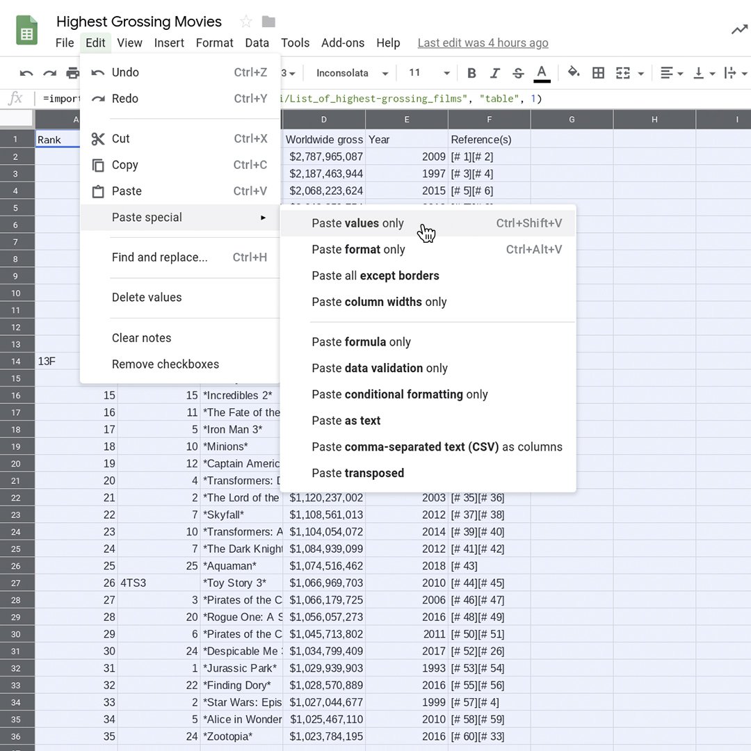
This table shows the result of importHTML. In this form, any changes to the data source (the Wikipedia page) will automatically be reflected here, and are updated at least once an hour. However, we can’t edit the values in the cells to remove undesired characters. We will use paste special in Google Sheets to create a static snapshot of the data. With this, we will lose the ability to update the table automatically via importHTML, but we will be able to edit it.
Select all of the data by left-clicking in the top left rectangle in your sheet. Once all cells are highlighted, click Edit > Copy. Select Edit > Paste special > Paste values only. We’re now able to edit the table.
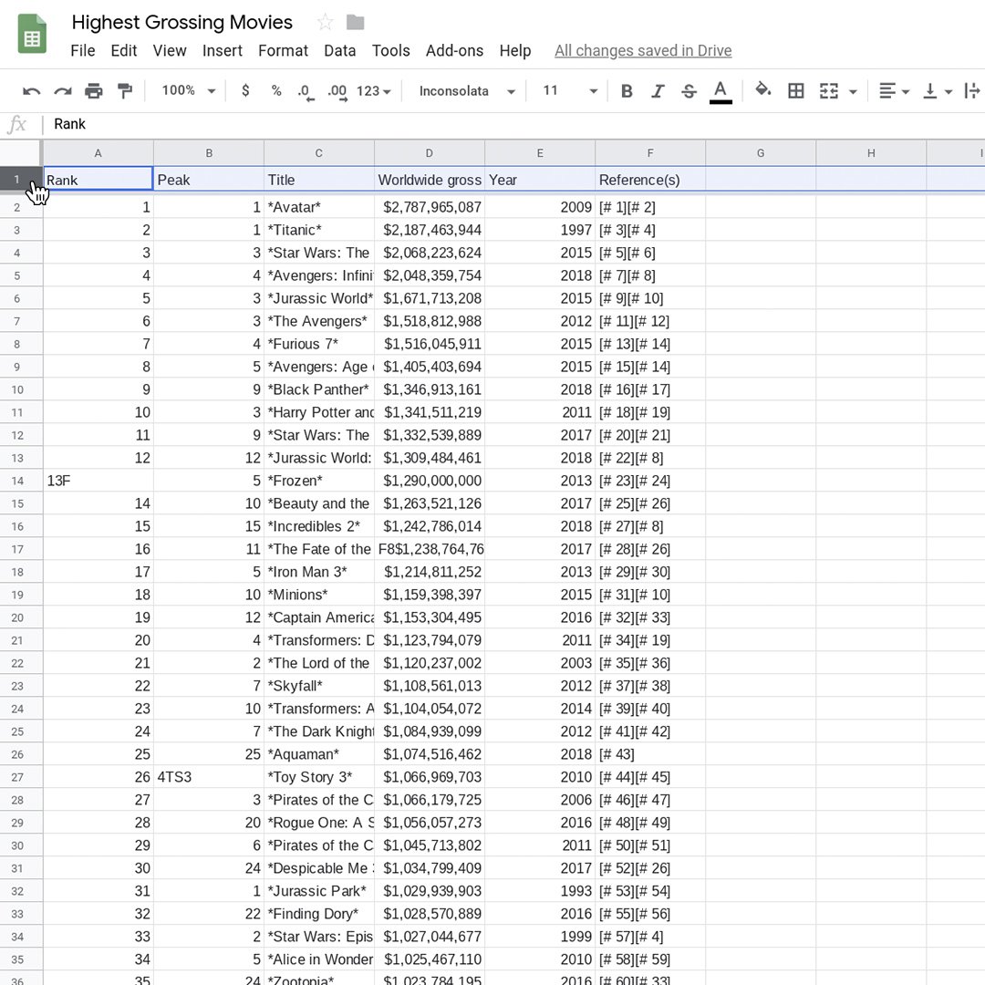
To make editing easier, we’ll freeze the row with the names of the columns. Hover the mouse cursor to the line just above row 1 over the gray bar. You will notice the cursor turns into a glove. Drag the bar to the bottom of row 1 and leave it there. Now the top row is frozen.
Editing the data.
importHTML will import leftover characters from the Wikipedia table that are useful for humans, but not computers. Let’s remove them and make our table cleaner!
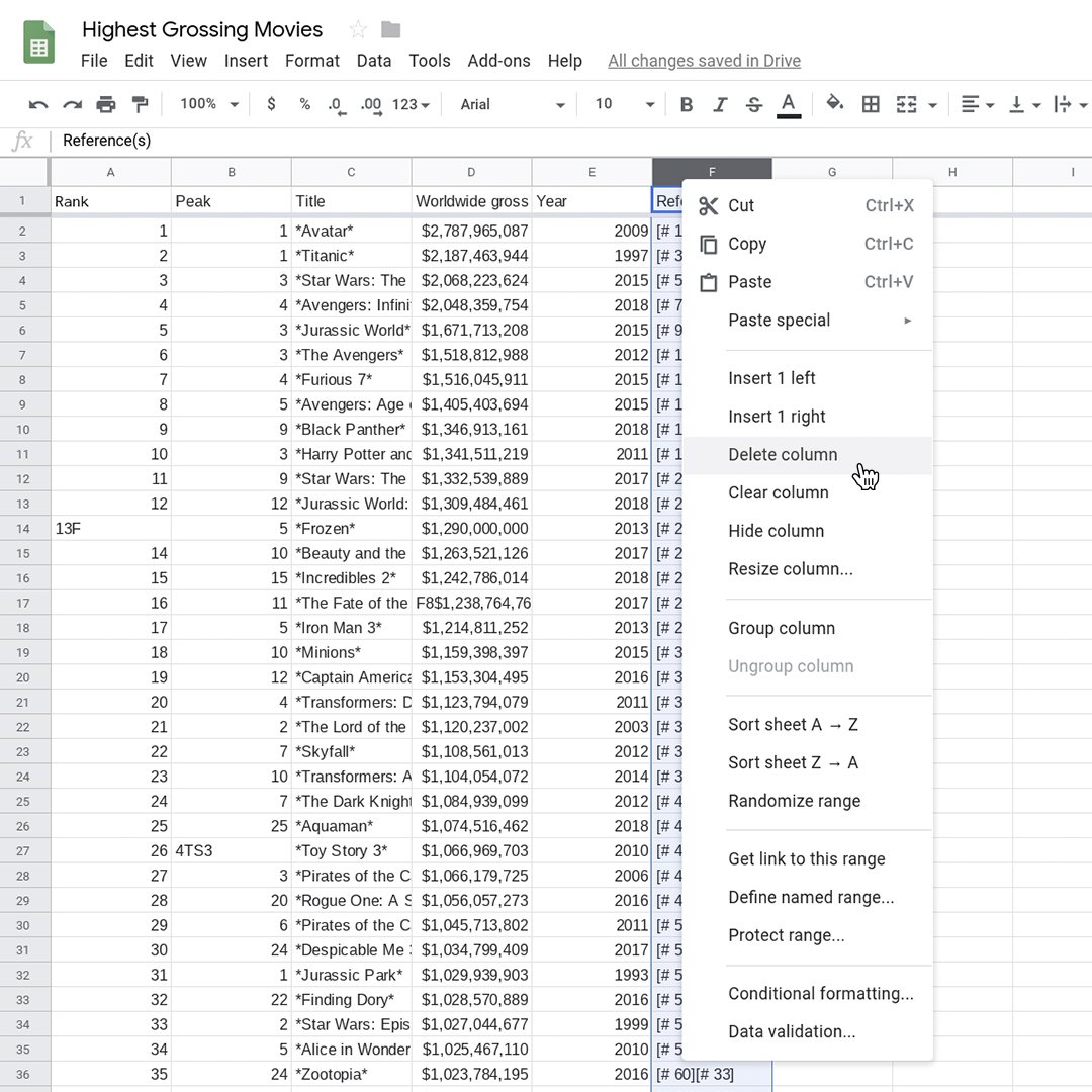
Since we don’t need column F for this exercise, right-click on the letter F at the top of the column and select Delete.
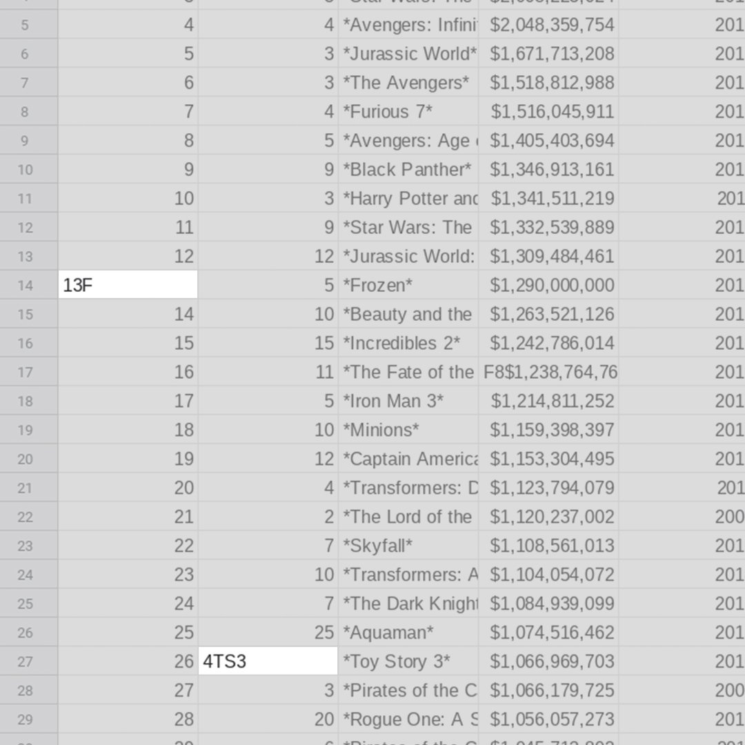
There is a letter “F” next to number 13 in row A14, and a “TS3” next to number 4 in cell B27. We will remove these characters so that only the numbers 13 and 4 remain.
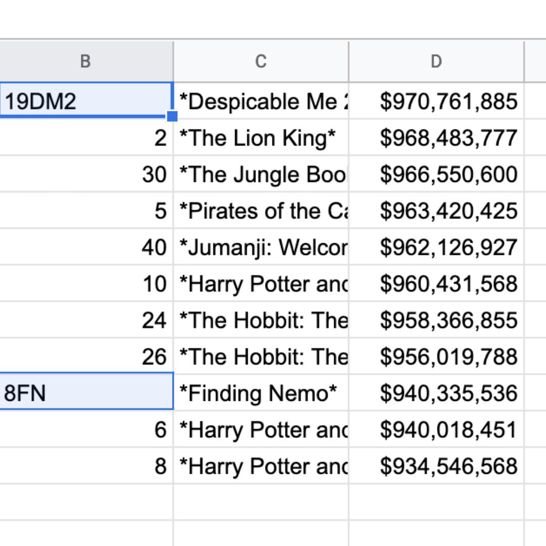
Remove the extra letters in cells B40 and B48, so that only 19 and 8 remain. Do the same in D17 to remove the leading “F8”.
Batch editing with Find and replace.
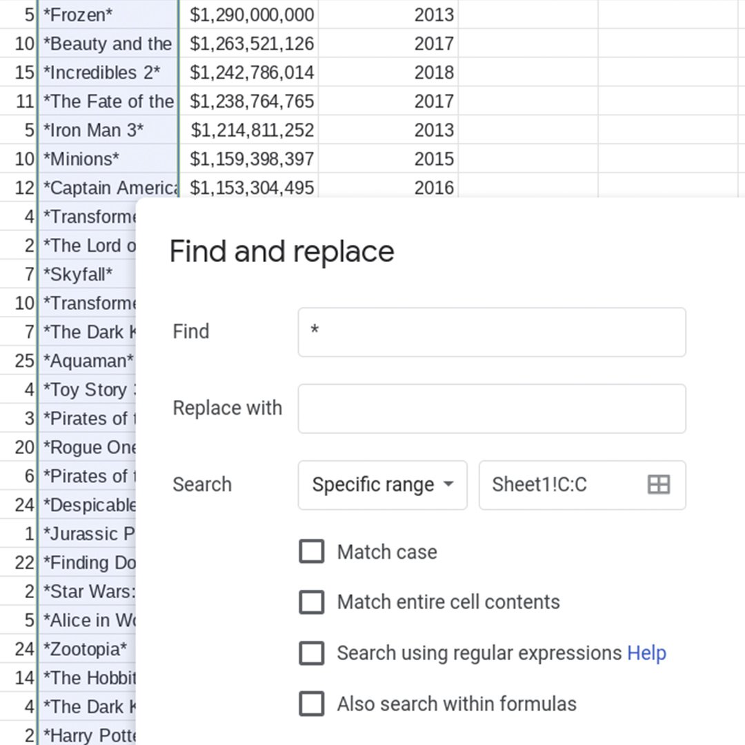
Now, take a look at column C. Let’s remove the leading and trailing * characters in a batch, rather than row by row, using the Find and replace feature.
Select column C by left-clicking on the letter C at the top of the column. Select Edit > Find and replace.
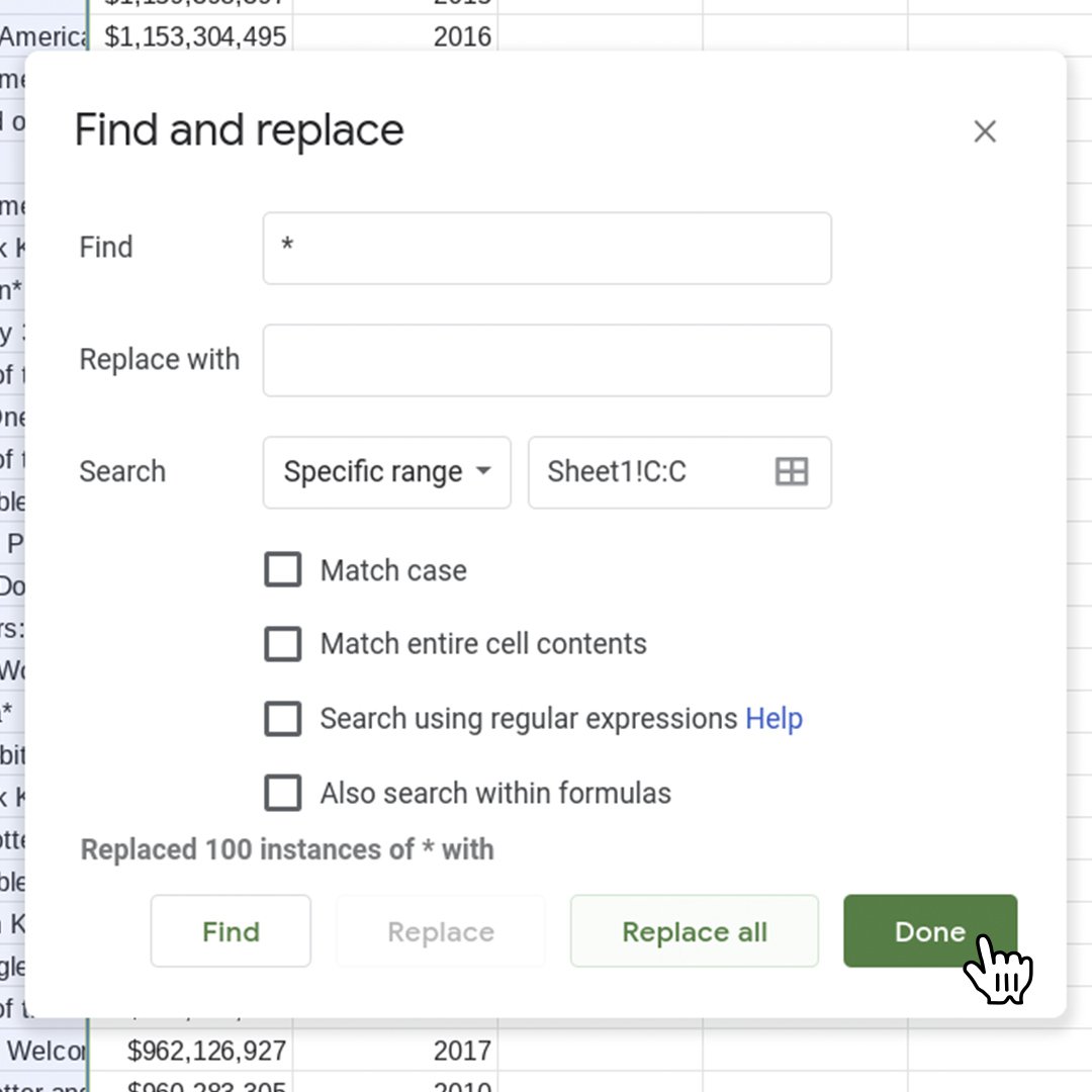
In the first text box type the asterisk symbol: * (that’s the character we want to find in column C). Leave the Replace with text box empty so that the asterisks get replaced with nothing, which means they will be deleted.
Make sure the Search option says Specific range and the range reflects the column you just selected. Leave the checkboxes unchecked.
Select Replace all. Notice Google Sheets will tell you it Replaced 100 instances of * with (nothing). That means you successfully removed 100 characters in 50 rows with just a few clicks!
Select Done. Our table is now clean and ready for us to work with. In the next lesson, we will produce visualizations and get insights from the data.
Congratulations!
You completed “Google Sheets: Cleaning data.”
To continue building your digital journalism skills and work toward Google News Initiative certification, go to our Training Center website and take another lesson:
For more Data Journalism lessons, visit:
newsinitiative.withgoogle.com/training/course/data-journalism